执行模式 1、Eager Execution:TensorFlow 2.0默认开启。类似于 python 这样的命令式编程,写好程序之后,不需要编译,就可以直接运行了,而且非常直观。
1
2
3
4
5
6
7
8
import tensorflow as tfprint (tf.executing_eagerly())v1 = [[2. ]] m = tf.matmul(v1, v1) print ("v1*v1, {}" .format (m))
2、Graph Execution:预先定义计算图,运行时反复使用,不能改变.适合大规模部署,适合嵌入式平台.Session 用来给定 Graph 的输入,指定 Graph 中的结果获取方式, 并启动数据在 Graph 中的流动.
1
2
3
4
5
6
7
8
9
10
11
12
13
14
15
16
import tensorflow.compat.v1 as tftf.disable_eager_execution() a = tf.constant(1 ) b = tf.constant(1 ) c = a + b sess = tf.Session() c_ = sess.run(c) print (c_)
启用 Eager Execution 会改变 TensorFlow 运算的行为方式 - 现在它们会立即评估并将值返回给 Python. 由于无需构建计算图并稍后在会话中运行,可以轻松使用 print() 或调试程序检查结果。评估、输出和检查张量值不会中断计算梯度的流程。
即使没有训练,也可以在 Eager Execution 中调用模型并检查输出:
1
2
3
4
5
6
7
8
9
10
11
12
13
14
15
16
17
18
19
20
21
22
23
24
import tensorflow as tf(mnist_images, mnist_labels), _ = tf.keras.datasets.mnist.load_data() dataset = tf.data.Dataset.from_tensor_slices( (tf.cast(mnist_images[..., tf.newaxis] / 255 , tf.float32), tf.cast(mnist_labels, tf.int64))) dataset = dataset.shuffle(1000 ).batch(32 ) mnist_model = tf.keras.Sequential([ tf.keras.layers.Conv2D(16 , [3 , 3 ], activation='relu' , input_shape=(None , None , 1 )), tf.keras.layers.Conv2D(16 , [3 , 3 ], activation='relu' ), tf.keras.layers.GlobalAveragePooling2D(), tf.keras.layers.Dense(10 ) ]) for images, labels in dataset.take(1 ): print ("Logits: " , mnist_model(images[0 :1 ]).numpy())
张量与变量 Tensor张量是具有统一类型(称为 dtype)的多维数组。张量与 np.arrays 有一定的相似性,所有张量都是不可变的,永远无法更新张量的内容,只能创建新的张量。
1
2
3
4
5
6
7
8
9
10
11
import tensorflow as tfrank_2_tensor = tf.constant([[1 , 2 ], [3 , 4 ], [5 , 6 ]], dtype=tf.float16) print (rank_2_tensor)
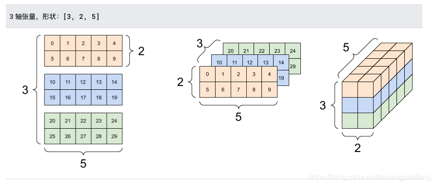
张量的轴可能更多,下面是一个包含 3 个轴的张量:
1
2
3
4
5
6
7
8
9
10
11
12
13
14
15
16
17
18
19
20
import tensorflow as tfrank_3_tensor = tf.constant([ [[0 , 1 , 2 , 3 , 4 ], [5 , 6 , 7 , 8 , 9 ]], [[10 , 11 , 12 , 13 , 14 ], [15 , 16 , 17 , 18 , 19 ]], [[20 , 21 , 22 , 23 , 24 ], [25 , 26 , 27 , 28 , 29 ]], ]) print (rank_3_tensor)
对于包含 2 个以上的轴的张量,您可以通过多种方式加以呈现。
通过使用 np.array 或 tensor.numpy 方法,您可以将张量转换为 NumPy 数组:
1
2
np.array(rank_2_tensor) rank_2_tensor.numpy()
各种运算 (op) 都可以使用张量。
1
2
3
4
5
6
7
8
9
10
11
12
13
14
c = tf.constant([[4.0 , 5.0 ], [10.0 , 1.0 ]]) print (tf.reduce_max(c))print (tf.argmax(c))print (tf.nn.softmax(c))
张量详情:
1
2
3
4
5
6
7
8
9
10
11
12
13
14
15
16
17
18
19
20
21
22
23
24
25
26
27
28
29
30
31
32
33
34
35
36
37
38
39
40
41
42
43
44
45
import tensorflow as tfrank_4_tensor = tf.zeros([3 , 2 , 4 , 5 ], dtype=tf.float64) print (rank_4_tensor)print ("Type of every element:" , rank_4_tensor.dtype) print ("Number of dimensions:" , rank_4_tensor.ndim) print ("Shape of tensor:" , rank_4_tensor.shape) print ("Elements along axis 0 of tensor:" , rank_4_tensor.shape[0 ]) print ("Elements along the last axis of tensor:" , rank_4_tensor.shape[-1 ]) print ("Total number of elements (3*2*4*5): " , tf.size(rank_4_tensor).numpy())
稀疏张量
在某些情况下,数据很稀疏,比如说在一个非常宽的嵌入空间中。为了高效存储稀疏数据,TensorFlow 支持 tf.sparse.SparseTensor
1
2
3
4
5
6
7
8
9
10
import tensorflow as tfsparse_tensor = tf.sparse.SparseTensor(indices=[[0 , 0 ], [1 , 2 ]], values=[1 , 2 ], dense_shape=[3 , 4 ]) print (sparse_tensor, "\n" )print (tf.sparse.to_dense(sparse_tensor))
变量 是用于表示程序处理的共享持久状态的推荐方法.
变量与张量的定义方式和操作行为都十分相似,实际上,它们都是 tf.Tensor 支持的一种数据结构。与张量类似,变量也有 dtype 和形状,并且可以导出至 NumPy.
1
2
3
4
5
6
7
8
9
10
11
12
import tensorflow as tfmy_tensor = tf.constant([[1.0 , 2.0 ], [3.0 , 4.0 ]]) my_variable = tf.Variable(my_tensor) bool_variable = tf.Variable([False , False , False , True ]) complex_variable = tf.Variable([5 + 4j , 6 + 1j ]) print ("Shape: " , my_variable.shape)print ("DType: " , my_variable.dtype)print ("As NumPy: " , my_variable.numpy)
变量张量互相转化。
1
2
3
4
5
6
7
8
9
10
11
import tensorflow as tfmy_tensor = tf.constant([[1.0 , 2.0 ], [3.0 , 4.0 ]], dtype=tf.float64) my_variable = tf.Variable(my_tensor) print ("A variable:" , my_variable) print ("\nViewed as a tensor:" , tf.convert_to_tensor(my_variable)) print ("\nIndex of highest value:" , tf.argmax(my_variable))print ("\nCopying and reshaping: " , tf.reshape(my_variable, ([1 , 4 ])))
在基于 Python 的 TensorFlow 中,tf.Variable 实例与其他 Python 对象的生命周期相同。如果没有对变量的引用,则会自动将其解除分配。
为了提高性能,TensorFlow 会尝试将张量和变量放在与其 dtype 兼容的最快设备上。这意味着如果有 GPU,那么大部分变量都会放置在 GPU 上。
可以手动放置变量:
1
2
3
4
5
6
7
8
9
10
11
12
import tensorflow as tfwith tf.device('CPU:0' ): a = tf.Variable([[1.0 , 2.0 , 3.0 ], [4.0 , 5.0 , 6.0 ]]) b = tf.Variable([[1.0 , 2.0 , 3.0 ]]) with tf.device('GPU:0' ): k = a * b print (k)
自动微分 TensorFlow 为自动微分提供了 tf.GradientTape API;即计算某个计算相对于某些输入(通常是 tf.Variable)的梯度。
1
2
3
4
5
6
7
8
9
10
import tensorflow as tfx = tf.Variable(3.0 ) with tf.GradientTape() as tape: y = x ** 2 dy_dx = tape.gradient(y, x) print (dy_dx.numpy())
上方示例使用标量,但是 tf.GradientTape 在任何张量上都可以轻松运行.
在大多数情况下,需要计算相对于模型的可训练变量的梯度。
1
2
3
4
5
6
7
8
9
10
11
12
13
14
15
import tensorflow as tflayer = tf.keras.layers.Dense(2 , activation='relu' ) x = tf.constant([[1. , 2. , 3. ]]) with tf.GradientTape() as tape: y = layer(x) loss = tf.reduce_mean(y ** 2 ) grad = tape.gradient(loss, layer.trainable_variables) for var, g in zip (layer.trainable_variables, grad): print (f'{var.name} , shape: {g.shape} ' )
1
2
3
4
5
6
7
8
9
10
11
import tensorflow as tfx = tf.constant([1 , 3.0 ]) with tf.GradientTape(persistent=True ) as tape: tape.watch(x) y = x * x z = y * y print (tape.gradient(z, x).numpy()) print (tape.gradient(y, x).numpy())
图和函数 tf.Graph与tf.function,计算图是一种数据结构,包含了一系列tf.Operation,这些tf.Operation被表示为计算节点,还包含了一系列tf.Tensor
可以使用tf.function来创建和使用计算图,tf.function可以将一个普通的Python函数封装成Tensorflow Function。Function可以像使用普通函数一样被调用,但其底层是封装了多个tf.Graph API来实现的 。
1
2
3
4
5
6
7
8
9
10
11
12
13
14
15
16
17
18
19
20
21
22
import tensorflow as tfdef a_regular_function (x, y, b ): x = tf.matmul(x, y) x = x + b return x a_function_that_uses_a_graph = tf.function(a_regular_function) x1 = tf.constant([[1.0 , 2.0 ]]) y1 = tf.constant([[2.0 ], [3.0 ]]) b1 = tf.constant(4.0 ) orig_value = a_regular_function(x1, y1, b1).numpy() tf_function_value = a_function_that_uses_a_graph(x1, y1, b1).numpy() print (orig_value == tf_function_value)
也可以使用@tf.function注解来标注计算图,并且可以让其内部调用的函数也使用计算图.
1
2
3
4
5
6
7
8
9
10
11
12
13
import tensorflow as tf@tf.function def my_relu (x ): return tf.maximum(0. , x) print (my_relu(tf.constant(5.5 )))print (my_relu([1 , -1 ]))print (my_relu(tf.constant([3. , -3. ])))
TF 2.0的其中一个重要改变就是去除tf.Session,在TF 2.0里面, 如果需要构建计算图, 只需要给python函数加上@tf.function的装饰器。
静态图的执行效率更高, 但是加速并不是一定的. 一般来说, 计算图越复杂, 加速效果越明显. 对于复杂的计算图, 比如训练深度学习模型, 获得的加速是巨大的. 如果某一部分的计算有复杂的计算图, 那么加速会比较明显, 但是很多时候, 比如一般的CNN模型, 主要计算量并不在于图的复杂性, 而在于卷积、矩阵乘法等操作, 加速并不会很明显.
小的数据计算量不足以覆盖生成图带来的消耗。
1
2
3
4
5
6
7
8
9
10
11
12
13
14
15
16
17
18
19
import tensorflow as tfimport timeitx = tf.random.uniform(shape=[10 , 10 ], minval=-1 , maxval=2 , dtype=tf.dtypes.int32) def power (x, y ): result = tf.eye(10 , dtype=tf.dtypes.int32) for _ in range (y): result = tf.matmul(x, result) return result print ("Eager execution:" , timeit.timeit(lambda : power(x, 100 ), number=1000 ))power_as_graph = tf.function(power) print ("Graph execution:" , timeit.timeit(lambda : power_as_graph(x, 100 ), number=1000 ))
模块、层和模型 在 TensorFlow 中,层和模型的大多数高级实现(例如 Keras 或 Sonnet)都在以下同一个基础类上构建:tf.Module。
tf.Module 是 tf.keras.layers.Layer 和 tf.keras.Model 的基类。
1
2
3
4
5
6
7
8
9
10
11
12
13
14
15
16
17
18
19
20
21
22
23
24
25
26
27
28
29
30
31
32
33
import tensorflow as tfclass Dense (tf.Module): def __init__ (self, in_features, out_features, name=None ): super ().__init__(name=name) self .w = tf.Variable( tf.random.normal([in_features, out_features]), name='w' ) self .b = tf.Variable(tf.zeros([out_features]), name='b' ) def __call__ (self, x ): y = tf.matmul(x, self .w) + self .b return tf.nn.relu(y) class MySequentialModule (tf.Module): def __init__ (self, name=None ): super ().__init__(name=name) self .dense_1 = Dense(in_features=3 , out_features=3 ) self .dense_2 = Dense(in_features=3 , out_features=2 ) @tf.function def __call__ (self, x ): x = self .dense_1(x) return self .dense_2(x) my_model = MySequentialModule(name="the_model" ) print (my_model([[2.0 , 2.0 , 2.0 ]]))print (my_model([[[2.0 , 2.0 , 2.0 ], [2.0 , 2.0 , 2.0 ]]]))
Keras 层,tf.keras.layers.Layer 是所有 Keras 层的基类,它继承自 tf.Module。只需换出父项,然后将 __call__ 更改为 call 即可将模块转换为 Keras 层
1
2
3
4
5
6
7
8
9
10
11
12
13
14
class MyDense (tf.keras.layers.Layer): def __init__ (self, in_features, out_features, **kwargs ): super ().__init__(**kwargs) self .w = tf.Variable( tf.random.normal([in_features, out_features]), name='w' ) self .b = tf.Variable(tf.zeros([out_features]), name='b' ) def call (self, x ): y = tf.matmul(x, self .w) + self .b return tf.nn.relu(y) simple_layer = MyDense(name="simple" , in_features=3 , out_features=3 )
Keras 模型定义为嵌套的 Keras 层,Keras 还提供了称为 tf.keras.Model 的全功能模型类 。它继承自 tf.keras.layers.Layer,因此 Keras 模型是一种 Keras 层,支持以同样的方式使用、嵌套和保存。Keras 模型还具有额外的功能,这使它们可以轻松训练、评估、加载、保存,甚至在多台机器上进行训练。
1
2
3
4
5
6
7
8
9
10
11
12
13
14
15
16
17
class MySequentialModel (tf.keras.Model): def __init__ (self, name=None , **kwargs ): super ().__init__(**kwargs) self .dense_1 = FlexibleDense(out_features=3 ) self .dense_2 = FlexibleDense(out_features=2 ) def call (self, x ): x = self .dense_1(x) return self .dense_2(x) my_sequential_model = MySequentialModel(name="the_model" ) print ("Model results:" , my_sequential_model(tf.constant([[2.0 , 2.0 , 2.0 ]])))
Keras 模型也可以使用 tf.saved_models.save() 保存,因为它们是模块。但是,Keras 模型具有更方便的方法和其他功能。
1 2 3 my_sequential_model.save("exname_of_file" ) reconstructed_model = tf.keras.models.load_model("exname_of_file" ) reconstructed_model(tf.constant([[2.0 , 2.0 , 2.0 ]]))
模型训练 解决一个机器学习问题通常包含以下步骤:
获得训练数据。
定义模型。
定义损失函数。
遍历训练数据,从目标值计算损失。
计算该损失的梯度,并使用optimizer 调整变量以适合数据。
计算结果。
开发一个简单的线性模型,
TensorFlow中几乎每个输入数据都是由张量表示,并且通常是向量。监督学习中,输出(即想到预测值)同样是个张量。
定义模型:
1
2
3
4
5
6
7
8
9
10
11
12
13
14
15
16
17
18
19
20
21
22
import tensorflow as tfclass MyModel (tf.Module): def __init__ (self, **kwargs ): super ().__init__(**kwargs) self .w = tf.Variable(5.0 ) self .b = tf.Variable(0.0 ) def __call__ (self, x ): return self .w * x + self .b model = MyModel() print ("Variables:" , model.variables)print (model(3.0 ).numpy() == 15.0 )
定义损失函数
损失函数衡量给定输入的模型输出与目标输出的匹配程度。目的是在训练过程中尽量减少这种差异。定义标准的L2损失,也称为“均方误差”:
1 2 3 def loss (target_y, predicted_y ): return tf.reduce_mean(tf.square(target_y - predicted_y))
定义训练循环
训练循环按顺序重复执行以下任务:
发送一批输入值,通过模型生成输出值
通过比较输出值与输出(标签),来计算损失值
使用梯度带(GradientTape)找到梯度值
使用这些梯度优化变量
tf.keras.optimizers中有许多梯度下降的变量,这里 借助tf.GradientTape的自动微分和tf.assign_sub的递减值(结合了tf.assign和tf.sub)实现
1 2 3 4 5 6 7 8 9 10 11 12 13 def train (model, x, y, learning_rate ): with tf.GradientTape() as t: current_loss = loss(y, model(x)) dw, db = t.gradient(current_loss, [model.w, model.b]) model.w.assign_sub(learning_rate * dw) model.b.assign_sub(learning_rate * db)
可以发送同一批* x 和 y * 经过循环训练,同时查看W和b的变化情况
1
2
3
4
5
6
7
8
9
10
11
12
13
14
15
16
17
18
19
20
model = MyModel() Ws, bs = [], [] epochs = range (10 ) def training_loop (model, x, y ): for epoch in epochs: train(model, x, y, learning_rate=0.1 ) Ws.append(model.w.numpy()) bs.append(model.b.numpy()) current_loss = loss(y, model(x)) print ("Epoch %2d: W=%1.2f b=%1.2f, loss=%2.5f" % (epoch, Ws[-1 ], bs[-1 ], current_loss))
使用Keras完成相同的解决方案
可以使用Keras的内置功能作为捷径,而不必在每次创建模型时都编写新的训练循环。
需要使用 model.compile() 去设置参数, 使用model.fit() 进行训练。借助Keras实现L2损失和梯度下降需要的代码量更少.
1
2
3
4
5
6
7
8
9
10
11
12
13
14
15
16
17
18
19
20
21
22
23
24
25
26
27
28
29
30
31
32
33
import tensorflow as tfclass MyModelKeras (tf.keras.Model): def __init__ (self, **kwargs ): super ().__init__(**kwargs) self .w = tf.Variable(5.0 ) self .b = tf.Variable(0.0 ) def __call__ (self, x, **kwargs ): return self .w * x + self .b keras_model = MyModelKeras() keras_model.compile ( run_eagerly=False , optimizer=tf.keras.optimizers.SGD(learning_rate=0.1 ), loss=tf.keras.losses.mean_squared_error, ) print (x.shape[0 ])keras_model.fit(x, y, epochs=10 , batch_size=1000 )
高级自动微分 如果不希望在模型中间对复杂运算微分,这可能有助于减少开销。其中可能包括计算指标或中间结果:
1
2
3
4
5
6
7
8
9
10
11
12
13
14
15
16
import tensorflow as tfx = tf.Variable(2.0 ) y = tf.Variable(3.0 ) with tf.GradientTape() as t: x_sq = x * x with t.stop_recording(): y_sq = y * y z = x_sq + y_sq grad = t.gradient(z, {'x' : x, 'y' : y}) print ('dz/dx:' , grad['x' ]) print ('dz/dy:' , grad['y' ])
tf.stop_gradient 函数更加精确。它可以用来阻止梯度沿着特定路径流动.
1
2
3
4
5
6
7
8
9
10
11
x = tf.Variable(2.0 ) y = tf.Variable(3.0 ) with tf.GradientTape() as t: y_sq = y**2 z = x**2 + tf.stop_gradient(y_sq) grad = t.gradient(z, {'x' : x, 'y' : y}) print ('dz/dx:' , grad['x' ]) print ('dz/dy:' , grad['y' ])
不规则张量 数据有多种形状;张量也应当有多种形状.包括:
可变长度特征,例如电影的演员名单。
成批的可变长度顺序输入,例如句子或视频剪辑。
分层输入,例如细分为节、段落、句子和单词的文本文档。
结构化输入中的各个字段,例如协议缓冲区。
有一百多种 TensorFlow 运算支持不规则张量,包括数学运算(如 tf.add 和 tf.reduce_mean)、数组运算(如 tf.concat 和 tf.tile)、字符串操作运算(如 tf.substr)、控制流运算(如 tf.while_loop 和 tf.map_fn)等:
1
2
3
4
5
6
7
8
digits = tf.ragged.constant([[3 , 1 , 4 , 1 ], [], [5 , 9 , 2 ], [6 ], []]) words = tf.ragged.constant([["So" , "long" ], ["thanks" , "for" , "all" , "the" , "fish" ]]) print (tf.add(digits, 3 ))print (tf.reduce_mean(digits, axis=1 ))print (tf.concat([digits, [[5 , 3 ]]], axis=0 ))print (tf.tile(digits, [1 , 2 ]))print (tf.strings.substr(words, 0 , 2 ))print (tf.map_fn(tf.math.square, digits))
许多 TensorFlow API 都支持不规则张量,包括 Keras、Dataset、tf.function、SavedModel 和 tf.Example
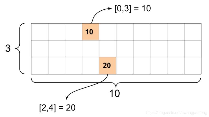
稀疏张量 tf.SparseTensor指定稀疏张量
1
2
3
4
5
6
7
8
import tensorflow as tfst1 = tf.SparseTensor(indices=[[0 , 3 ], [2 , 4 ]], values=[10 , 20 ], dense_shape=[3 , 10 ]) print (st1)
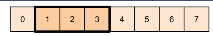
Tensor切片 1 2 3 4 5 6 7 8 9 10 11 import tensorflow as tft1 = tf.constant([0 , 1 , 2 , 3 , 4 , 5 , 6 , 7 ]) print (tf.slice (t1, begin=[1 ], size=[3 ])) print (t1[1 :4 ])